Basic CWT_Multi theory
On this page we provide the basic theory required to understand how CWT_Multi works. This knowledge empowers the user to get the most out of CWT_Multi for their specific application. We present ideas and illustrations, rather than comprehensive maths. Future pages in this documentation will cover the mathematic details. For now, we refer the reader to Lobo et al. (2024) and references therein.
We briefly cover some basic preliminaries before diving into the details of CWT_Multi.
Tidal species and constituents
Different tidal constituents describe unique frequencies of tidal forcing that correspond to different sets of Doodson numbers, i.e., different combinations of tidal forcing phenomena that lead to a unique frequency. Doodson numbers describe the fundamental forcing temporal periods of the tides. (The first Doodson number describes number of cycles per lunar day, the second Doodson number describes number of cycles per sidereal year, etc.) Tidal species describes groups of tidal constituents that have the same number of cycles per lunar day, i.e, they share a first Doodson number.
The Rayleigh criterion defined
The Rayleigh criterion, \(R_{C}\), describes the minimum analysis window length required to separate two signals with different frequencies. That is, the minimum window length is
\[L_{w} = R_{C} \, \left | f_{1} - f_{2} \right | ^{-1} \ \mathrm{seconds} \, ,\]
where we generally require \(R_{C} = 1\). For example, in order to resolve the \(M_{2}\) and \(S_{2}\) tidal constituents with \(R_{C}=1\), we need to use an analysis window length of
\[\begin{split}L_{w} &= \left | f_{M_{2}} - f_{S_{2}} \right | ^{-1} \\ &= \left | 1/12.4206012 - 1/12 \right | ^{-1} \ \mathrm{hr} \\ &\approx 15 \ \mathrm{days} \, .\end{split}\]
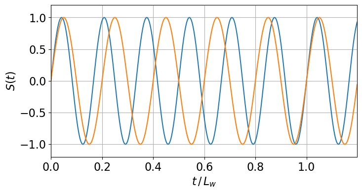
Another way to word the Rayleigh criterion is: if a signal is composed of sine waves at two different frequencies, we need the sine wave at the higher frequency to complete at least one more cycle than the sine wave at the lower frequency, in order to be able to tell the two frequencies apart. This is shown graphically below.
The Rayleigh criterion in spectral space
A useful way to think of the Rayleigh criterion is in terms of spectra. A spectrum is a measure of a quantity as a function of frequency, e.g., power spectrum, absorption spectrum. Thus, we can draw a spectrum where the x-axis is frequency, and the y-axis is some measure of tidal amplitude.
Below we show the energy spectrum of a signal that is made up of the sum of equal-amplitude sine waves at the \(M_{2}\) and \(S_{2}\) tidal frequencies. We compute the energy spectrum (using the Fast Fourier Transform algorithm) for signals of three different lengths: \(L_{w} / 2\), \(L_{w}\), and \(2 \, L_{w}\), where \(L_{w}\) is the minimum window length required to separate the two frequencies, as defined by the Rayleigh criterion. We find that with the shortest window we are not able to differentiate between energy at the two frequencies (red line). Once we analyze a signal that is at least the length \(L_{w}\), we marginally resolve energy at the two frequencies (green line).
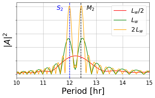
Note, however, that as the analyzed signal gets longer, the peaks at the two frequencies become more distinct (yellow line). If we had an infinitely long signal, the energy at the two frequencies would be represented by vertical lines (hence the often-used term line spectra). The apparent “spreading” of energy at frequencies around \(M_{2}\) and \(S_{2}\) is an artifact of the finite-length analysis window.
CWT_Multi application method for a full time series
The fundamental application of CWT_Multi is to define tidal amplitudes and phases that vary as functions of time. From these time-varying amplitudes and phases we can then reconstruct a nonstationary time series of water level data, for example. Here we provide a brief explanation of the framework used to accomplish this goal.
First, we note that CWT_Multi performs both a species and constituents analysis. The species analysis defines time-varying amplitudes and phases for each tidal species, i.e., diurnal (\(D_{1}\)), semidiurnal (\(D_{2}\)), etc. This analysis can resolve time-changes in species amplitudes on the order of a couple/few days.
The constituents analysis defines time-varying amplitudes and phases for 7-9 individual tidal constituents within the diurnal and semidiurnal tidal species bands. Since constituents within the same species are fairly close together (below, we will detail how the closeness of the \(M_{2}\) and \(S_{2}\) constituents affects our analysis, for example), we resolve time-changes of constituent amplitudes on the order of one to two weeks.
The main steps that the CWT_Multi analysis is comprised of are:
Define the analysis window for a given time step, centered on time \(t_m\)
Convolve each filter from the filter bank with data within the analysis window. (This step outputs a complex response.)
Solve the response coefficient matrix problem (detailed below).
Store complex solution for all frequencies that have corresponding filters at the time \(t_m\). (From this complex solution, one easily retrieves amplitude and phase.)
Move the analysis window forward to \(t_m \, + \, D_{f} \Delta t\), where \(D_{f}\) is the decimation factor, i.e., the number of time steps between adjacent CWT_Multi analyses, and \(\Delta t\) is the sampling period.
Repeat.
We now describe the maths behind the CWT_Multi process that occurs at each analysis time step, centered on \(t_m\).
CWT_Multi filters
The spectra shown above were constructed using Fourier transforms. The Fourier amplitude at a given frequency, \(f\), is essentially the magnitude of the convolution of a complex sinusoid, of the form
\[e^{i \,2 \pi f t} = \mathrm{cos}(2 \pi f t ) + i \, \mathrm{sin} (2 \pi f t ) \, ,\]
with the signal being analyzed, over the analysis window length. The complex output then contains the information necessary to find the amplitude and phase of the signal at the frequency \(f\).
CWT_Multi performs analogous convolutions using complex wavelet filters. An example of such a filter is shown below.
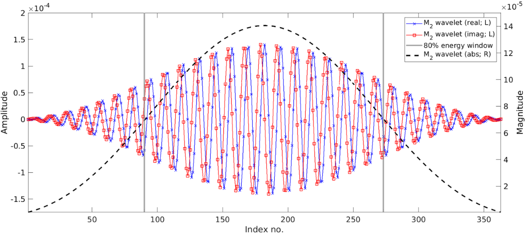
In short, the form of our wavelet maximizes the amount of information one is able to extract from this convolution given a finite analysis window length. However, the optimal form of wavelets are a topic of active research, and always require some trade-off (see Lilly and Ohelde 2012).
CWT_Multi defines wavelets at frequencies where tidal energy is expected, and then constructs a matrix problem for the complex convolution output. This matrix problem allows for resolution of frequencies for analysis windows of lengths that violate the Rayleigh criterion. We will soon present the assumptions and methods of the response coefficient matrix. First, we must understand what a frequency response is, and how this concept manifests in CWT_Multi.
Frequency response: A definition
From the spectrum plot above, we see that finite-length complex sinusoids (and wavelet filters) within a given frequency band, which we define as \(f \pm \Delta f\), will “respond” to energy at the central frequency, \(f\). For example, in the spectra above, computed using the FFT, there is apparent energy at frequencies surrounding the \(M_{2}\) and \(S_{2}\) frequencies, even though our analyzed signal is only comprised of two sine waves.
Importantly, this frequency response is a function of the analysis window length. Shorter filters (equivalently, shorter analysis windows) will increase the frequency range, \(\Delta f\), at which the filter will respond to energy at adjacent frequencies.
CWT_Multi leverages the frequency response of filters centered on tidal frequencies to energy at adjacent tidal frequencies to construct a matrix problem. We now present this matrix problem.
Response coefficient matrix: The problem
The response coefficient matrix problem is
\[\vec{f} (t_m) = \boldsymbol{R} \, \vec{a}(t_m) \, ,\]
where:
\(t_m\) is the time at the center of the analysis window
\(\vec{f}\) is an \(N \times 1\) column vector of the complex outputs from the \(N\) complex wavelet filters (at frequency \(f_n\)) with signal, centered on time \(t_m\)
\(\boldsymbol{R}\) is the response coefficient matrix (RCM), which we describe in detail below
\(\vec{a}(t_m)\) is the \(N \times 1\) column vector of the true amplitudes of the signal at the frequencies \(f_n\)
The easiest way to understand the RCM is in terms of a simplified problem. Consider a set of wavelet filters at the \(M_{2}\) and \(S_{2}\) frequencies, where we would like to define the \(M_{2}\) and \(S_{2}\) amplitudes as a function of time. We thus define the RCM as
\[\begin{split}\boldsymbol{R} = \begin{pmatrix} r_{M_{2}, \, M_{2}} & r_{M_{2}, \, S_{2}} \\ r_{S_{2}, \, M_{2}} & r_{S_{2}, \, S_{2}} \end{pmatrix} \, ,\end{split}\]
where \(r_{f_{1}, \, f_{2}}\) describes the frequency of the \(f_{1}\) filter to energy at the \(f_{2}\) frequency, with a maximum value of unity. For example, \(r_{M_{2}, \, M_{2}} = 1\), since the \(M_{2}\) filter will respond to all of the energy at the \(M_{2}\) frequency.
As noted above, the filter width in time (equivalently, the length of the analysis window), will determine the width in frequency-space, \(\Delta f\), at which the filter will respond to energy at adjacent frequencies. In particular, a wider frequency in time has a narrower response in frequency-space. We can now plot the frequency response for our simplified problem. In particular, we show the filter responses for the two filters for two different choices of wavelet filter length.
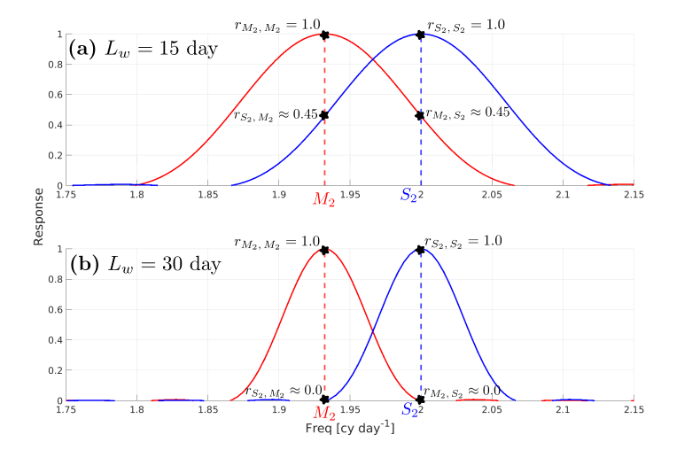
We show the frequency response for the \(M_{2}\) (red) and \(S_{2}\) (blue) filters above, as a function of frequency. For the narrower-in-time filters (panel (a)), the surrounding band of frequencies, for which the respective filters respond to energy, is relatively wide. In particular, \(r_{S_{2}, \, M_{2}} \approx 0.45\) means that the \(S_{2}\) filter will include 45% of the energy that exists at the \(M_{2}\) frequency in its estimate of the amplitude of the \(S_{2}\) component of the signal during the analysis window. Though this may seem like a problem, we will explain how the RCM accounts for such overlap in the following section. First, we review some salient aspects of the frequency response plot, and their connections to the RCM.
We have \(r_{M_{2}, \, M_{2}} = 1\) and \(r_{S_{2}, \, S_{2}} = 1\), as expected
If the \(M_{2}\) and \(S_{2}\) filters are the same length, as above, then we have \(r_{S_{2}, \, M_{2}} = r_{M_{2}, \, S_{2}}\), and the RCM is a symmetric matrix
The wider the filter in time, i.e., the longer the analysis window, the more narrow the frequency response is
The last point should be thought upon, as it is this feature of the RCM that guides one’s choice of filter lengths when using CWT_Multi. The user must choose a trade-off between having time-resolution (i.e., being able to define a tidal amplitude that varies as a function of time) and frequency-resolution (i.e., being able to distinguish energy between two frequencies.
Note
The reader might be wondering why the 15-day-long wavelet filters respond to nearby frequencies, whereas the Rayleigh criterion suggests that 15 days is long enough to resolve the \(M_{2}\) and \(S_{2}\) signals. This is because the wavelet filters are tapered, and carry about 80% of their energy in the middle half of the filter (see the plot of complex wavelet filter above). So the effective length of a wavelet filter, in terms of a Rayleigh criterion, is close to about half of the user-specified wavelet filter length.
Response coefficient matrix: The solution
We have defined the response coefficient matrix (RCM), and have hopefully provided some insight into its meaning and its connection to CWT_Multi analysis. As a final stop in our exposition of the theory that supports CWT_Multi analysis, we consider the solution to the RCM problem.
The RCM problem (also defined above) is
\[\vec{f} (t_m) = \boldsymbol{R} \, \vec{a}(t_m) \, ,\]
In the example currently under consideration, we consider filters only at the \(M_{2}\) and \(S_{2}\) tidal frequencies. Now, suppose that signal only has energy at the \(M_{2}\) and \(S_{2}\) frequencies, each with unity amplitude.
For filters that are 15 days long (panel (a)) above, our RCM problem becomes
\[\begin{split}\begin{pmatrix} 1.45 \\ 1.45 \\ \end{pmatrix} = \begin{pmatrix} 1.0 & 0.45 \\ 0.45 & 1.0 \end{pmatrix} \ \begin{pmatrix} a_{M_{2}} \\ a_{S_{2}} \end{pmatrix} \, .\end{split}\]
By multiplying both sides by \(\boldsymbol{R}^{-1}\) we find
\[\begin{split}\vec{a} = \begin{pmatrix} 1.0 \\ 1.0 \end{pmatrix} \, .\end{split}\]
Thus we are able to recover our true amplitudes, \(\vec{a}\), from (i) the response of our wavelet filters to the signal, and (ii) the known response coefficient matrix. Note that the RCM problem becomes trivial for \(r_{S_{2}, \, M_{2}} = r_{M_{2}, \, S_{2}} \approx 0.0\), where the filters do not respond to energy at the adjacent tidal frequency.
CWT_Multi creates an analogous matrix problem for tidal constituents within a tidal species band for the constituents analysis. An analogous matrix problem is also create for the species analysis, where there is only one filter per tidal species. However, these species filters are much shorter, and therefore have a much wider frequency response. That is, we favor resolution in time (i.e., a shorter filter can capture changes that occur on smaller time scales) and sacrifice frequency resolution (i.e., the species filter can only identify a “blob” of energy within each respective tidal species band).
The application of the CWT_Multi method to observed data is more unwieldy, because (i) there will exist energy at tidal frequencies that do not have filters, and (ii) as more frequencies are added to the filter bank, the RCM problem becomes more susceptible to “cross-talk” between tidal consituents/species. Regardless, Lobo et al., (2024) have shown that the CWT_Multi method is effective at quantifying nonstationary tidal amplitudes/phases and reconstructing a tidal-energy-only time series for many applications.
Additional reading
See Lobo et al., (2024) for details on the information presented on this page.
Lilly and Ohelde (2012) provides excellent exposition to the considerations had when choosing wavelet filter type and parameters.